1. The Simple Harmonic Oscillator

Here we will expand on the harmonic oscillator first shown in the getting started script. I’ll walk you through some of the features of desolver and hopefully give a better a sense of how to use the software.

So let’s begin!

First we import the libraries we’ll need. I import all the matplotlib machinery using the magic command %matplotlib, but this is only for notebook/ipython environments.

Then I import desolver and the desolver backend as well (this will be useful for specifying our problem), and set the default datatype to float64.

%matplotlib inline
from matplotlib import pyplot as plt

import desolver as de
import desolver.backend as D

D.set_float_fmt('float64')

Using numpy backend

1.1. Specifying the Dynamical System

Now let’s specify the right hand side of our dynamical system. It should be

\[\frac{\mathrm{d^2}x}{\mathrm{dt}^2} = -\frac{k}{m} x\]

But desolver only works with first order differential equations, thus we must cast this into a first order system before we can solve it. Thus we obtain the following system

\[\begin{split}\begin{array}{l} \frac{\mathrm{d}x}{\mathrm{dt}} = v_x \\ \frac{\mathrm{d}v_x}{\mathrm{dt}} = -\frac{k}{m} x \end{array}\end{split}\]

which can be specified as a simple matrix equation as

\[\begin{split}\begin{array}{c} \frac{\mathrm{d}y}{\mathrm{dt}} = \begin{bmatrix} 0 & 1 \\ -\frac{k}{m} & 0 \end{bmatrix} \cdot \vec y \\ \vec y = \begin{bmatrix}x \\ v_x\end{bmatrix} \end{array}\end{split}\]

@de.rhs_prettifier(
    equ_repr="[vx, -k*x/m]",
    md_repr=r"""
$$
\frac{\mathrm{d}y}{\mathrm{dt}} = \begin{bmatrix}
   0            & 1 \\
   -\frac{k}{m} & 0
   \end{bmatrix} \cdot \vec y
$$
"""
)
def rhs(t, state, k, m, **kwargs):
    return D.array([[0.0, 1.0], [-k/m,  0.0]])@state

First thing to notice is that we used the backend to specify the matrix and minimise the use of numpy specific machinery. This isn’t necessary if you only use numpy, but by doing this we can make this code run with the pytorch backend with minimal effort.

Second thing is the use of the decorator @de.rhs_prettifier, this is a convenience decorator that allows me to specify a text representation of the differential equations. Convenient if I want to print it

print(rhs)

[vx, -k*x/m]

Or if I want it to look pretty when it is rendered in the notebook

display(rhs)

\[\begin{split}\frac{\mathrm{d}y}{\mathrm{dt}} = \begin{bmatrix} 0 & 1 \\ -\frac{k}{m} & 0 \end{bmatrix} \cdot \vec y\end{split}\]

Let’s specify the initial conditions as well

y_init = D.array([1., 0.])

And now we’re ready to integrate!

1.2. The Numerical Integration

There are a number of things we must choose before we numerically integrate our system of equations. The first of these is whether or not we want an interpolating spline so that we can compute the state of our system between timesteps. The second is the duration of the numerical integration. And the third is the value of parameters of the system: k and m.

Unlike scipy, desolver let’s you specify a dictionary of constants that are passed to the rhs function and can be modified even after constructing the OdeSystem object. This is particularly useful if you want to vary a single constant over multiple integrations without changing any other parameters.

Now, we’ll set the numerical integration to 1 cycle of the oscillator at k=1 and m=1 which, when computed from the formula \(T=2\pi\sqrt{\frac{k}{m}}\), is exactly \(2\pi\).

a = de.OdeSystem(rhs, y0=y_init, dense_output=True, t=(0, 2*D.pi), dt=0.01, rtol=1e-9, atol=1e-9, constants=dict(k=1.0, m=1.0))

a.integrate()

Since k=1 and m=1 and we integrated for 1 cycle, we expect that the final state of the system is the same as the initial state.

print("initial state = {}".format(a[0].y))
print("final state   = {}".format(a[-1].y))
print("maximum absolute difference = {}".format(D.max(D.abs(a[-1].y - a[0].y))))

initial state = [1. 0.]
final state   = [ 1.00000000e+00 -1.14580831e-10]
maximum absolute difference = 3.2781628522826622e-09

Wonderful! We see that the final state is almost exactly the same. Furthermore, we see that this is within the tolerances we specified when creating the OdeSystem where we set rtol and atol to 1e-9.

To show you that this is not a fluke, we’ll change them to 1e-12 and see what happens.

a.rtol = 1e-12
a.atol = 1e-12
a.reset()
a.integrate()

print("initial state = {}".format(a[0].y))
print("final state   = {}".format(a[-1].y))
print("maximum absolute difference = {}".format(D.max(D.abs(a[-1].y - a[0].y))))

initial state = [1. 0.]
final state   = [ 1.00000000e+00 -2.88935542e-14]
maximum absolute difference = 3.255395952805884e-12

It’s very simple to change the tolerances and rerun the system. Furthermore, we can update our constants and see what happens.

If we quadruple k, the spring constant, the period will double, and so after an integration period of \(2\pi\) the system should, yet again, be in a final state that is almost exactly the initial state.

a.constants['k'] = a.constants['k'] * 4
a.reset()
a.integrate()

print("initial state = {}".format(a[0].y))
print("final state   = {}".format(a[-1].y))
print("maximum absolute difference = {}".format(D.max(D.abs(a[-1].y - a[0].y))))

initial state = [1. 0.]
final state   = [ 1.00000000e+00 -1.69420034e-13]
maximum absolute difference = 9.035661108214299e-12

The final state is again almost the same as the initial state, but now the maximum absolute difference has increased. This is due to the fact that the numerical error when using an adaptive runge-kutta method is not a random walk, but a function of the whole numerical procedure. Thus if we double the initial integration time, and set k=1 again, we’ll see that the error is larger.

a.constants['k'] = 1
a.tf = 4*D.pi
a.reset()
a.integrate()

print("initial state = {}".format(a[0].y))
print("final state   = {}".format(a[-1].y))
print("maximum absolute difference = {}".format(D.max(D.abs(a[-1].y - a[0].y))))

initial state = [1. 0.]
final state   = [ 1.00000000e+00 -5.68208675e-14]
maximum absolute difference = 6.517453243759519e-12

The longer we integrate for, the larger this error will become. Is there anything we can do?

YES

We can use a symplectic integrator since this is a system with a Hamiltonian \(H=\frac{kx^2}{2} + \frac{mv_x^2}/2\).

A symplectic integrator preserves the symplectic two-form \(\mathrm{d}\vec p \wedge\mathrm{d}\vec q\) where \(p\) is the momentum and \(q\) is the position such that

\[\begin{split}\begin{array}{l} \frac{\mathrm{d}p}{\mathrm{dt}} = -\frac{\partial H}{\partial q} \\ \frac{\mathrm{d}q}{\mathrm{dt}} = \frac{\partial H}{\partial p} \end{array}\end{split}\]

where, in our case, \(v_x = \frac{p}{m}\) and \(x = q\).

Why is this important? I’ll leave the detailed theory to Wikipedia and other sources, but the jist of it is that a symplectic integrator is essentially a geometric transformation in the phase space of the system and thus preserves the differential volume element of a Hamiltonian that is almost, but not quite, the Hamiltonian of the system.

This is great because it means that, in the best case scenario, the errors in the numerically integrated states are random walks instead of increasing linearly with the integration time. The downside is that a symplectic integrator is not adaptive and thus requires more function evaluations than a Runge-Kutta method.

a.set_method("BABS9O7H")
a.dt = 0.05
a.tf = 2*D.pi
a.integrate()

An integration was already run, the system will be reset

print("initial state = {}".format(a[0].y))
print("final state   = {}".format(a[-1].y))
print("maximum absolute difference = {}".format(D.max(D.abs(a[-1].y - a[0].y))))

initial state = [1. 0.]
final state   = [ 1.0000000e+00 -2.7269853e-15]
maximum absolute difference = 2.7269853042355408e-15

a.set_method("BABS9O7H")
a.dt = 0.05
a.tf = 8*D.pi
a.integrate()

An integration was already run, the system will be reset

print("initial state = {}".format(a[0].y))
print("final state   = {}".format(a[-1].y))
print("maximum absolute difference = {}".format(D.max(D.abs(a[-1].y - a[0].y))))

initial state = [1. 0.]
final state   = [ 1.00000000e+00 -9.48546797e-15]
maximum absolute difference = 9.485467966641181e-15

a.set_method("BABS9O7H")
a.dt = 0.05
a.tf = 32*D.pi
a.integrate()

An integration was already run, the system will be reset

print("initial state = {}".format(a[0].y))
print("final state   = {}".format(a[-1].y))
print("maximum absolute difference = {}".format(D.max(D.abs(a[-1].y - a[0].y))))

initial state = [1. 0.]
final state   = [ 1.00000000e+00 -4.41313652e-14]
maximum absolute difference = 4.413136522884997e-14

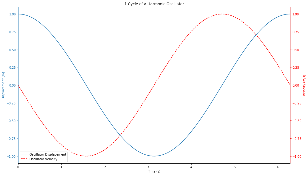
Above, I’ve run the numerical integration using a step size of \(0.05\) for increasing integration periods from one cycle to four cycles to sixteen cycles and, despite that, the error has stayed near the limits of double precision arithmetic. If I further integrate for 1024 cycles, we’ll see that the error begins to increase and this is expected because although the errors in each step may be random walks, they have a cumulative effect that is not necessarily a random walk.

a.set_method("BABS9O7H")
a.dt = 0.05
a.tf = 2*1024*D.pi
a.integrate()

An integration was already run, the system will be reset

print("initial state = {}".format(a[0].y))
print("final state   = {}".format(a[-1].y))
print("maximum absolute difference = {}".format(D.max(D.abs(a[-1].y - a[0].y))))

initial state = [1. 0.]
final state   = [ 1.00000000e+00 -2.06966388e-12]
maximum absolute difference = 2.069663884718409e-12

fig = plt.figure(figsize=(14,8))
ax  = fig.add_subplot(111)

displn = ax.plot(a.t, a.y[:, 0], label="Oscillator Displacement", color='C0')
axt = ax.twinx()
velln  = axt.plot(a.t, a.y[:, 1], label="Oscillator Velocity", color='red', linestyle='--')

ax.set_xlabel("Time (s)")
ax.set_ylabel("Displacement (m)")
axt.set_ylabel("Velocity (m/s)")
ax.set_xlim(0, 2*D.pi)

ax.spines['left'].set_color('C0')
ax.tick_params(axis='y', colors='C0')
ax.yaxis.label.set_color('C0')

axt.spines['right'].set_color('red')
axt.spines['left'].set_color('C0')
axt.tick_params(axis='y', colors='red')
axt.yaxis.label.set_color('red')

# added these three lines
lns = displn + velln
labs = [l.get_label() for l in lns]
ax.legend(lns, labs)

ax.set_title("1 Cycle of a Harmonic Oscillator")
plt.tight_layout()

1.3. Looking at the Hamiltonian

So we’ve said that a symplectic integrator preserves a perturbed Hamiltonian, we should be able to see this by computing the Hamiltonian at each timestep and looking at how it evolves over the course of a numerical integration.

Let’s first define the Hamiltonian.

def kinetic_energy(t, state, k, m):
    x, vx = state
    return m * vx**2 / 2

def potential_energy(t, state, k, m):
    x, vx = state
    return k * x**2 / 2

def hamiltonian(t, state, k, m):
    return kinetic_energy(t, state, k, m) + potential_energy(t, state, k, m)

Now it’s not interesting to just look at the Hamiltonian alone, we’d like to look at how the Hamiltonian evolves so we will look at the absolute difference between the Hamiltonian at time \(t\) and the initial Hamiltonian.

To start off, we’ll look at the Hamiltonian when we use an adaptive integrator.

a.reset()
a.method = "RK45"
a.rtol = 1e-9
a.atol = 1e-9
a.tf   = 4*2*D.pi
a.integrate()

fig = plt.figure(figsize=(14,8))
ax  = fig.add_subplot(111)

E_H = D.abs(hamiltonian(a.t, a.y.T, **a.constants) - hamiltonian(a.t[0], a.y[0], **a.constants))

disp_H = ax.plot(a.t, E_H, label="Hamiltonian / Total Energy", color='black')

ax.set_xlabel("Time (s)")
ax.set_ylabel("Hamiltonian (J)")

# added these three lines
ax.legend()
ax.set_yscale("log")

ax.set_title("{:.0f} Cycle{} of a Harmonic Oscillator".format(a.tf/(2*D.pi), "s" if a.tf/(2*D.pi) > 1 else ""))
plt.tight_layout()

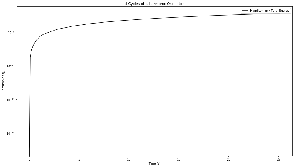
We see that the Hamiltonian starts off correctly, but then, very rapidly, jumps up to an error on the order of \(10^{-9}\) which is the same as the tolerance we’ve set for the numerical integration.

Now let’s compare this to a symplectic integrator.

a.reset()
a.set_method("BABS9O7H")
a.rtol = 1e-9
a.atol = 1e-9
a.dt   = 1e-1
a.tf   = 4*2*D.pi
a.integrate()

fig = plt.figure(figsize=(14,8))
ax  = fig.add_subplot(111)

E_H = D.abs(hamiltonian(a.t, a.y.T, **a.constants) - hamiltonian(a.t[0], a.y[0], **a.constants))

disp_H = ax.plot(a.t, E_H, label="Hamiltonian / Total Energy", color='C0')

ax.set_xlabel("Time (s)")
ax.set_ylabel("Hamiltonian (J)")

# added these three lines
ax.legend()
ax.set_yscale("log")

ax.set_title("{:.0f} Cycle{} of a Harmonic Oscillator".format(a.tf/(2*D.pi), "s" if a.tf/(2*D.pi) > 1 else ""))
plt.tight_layout()

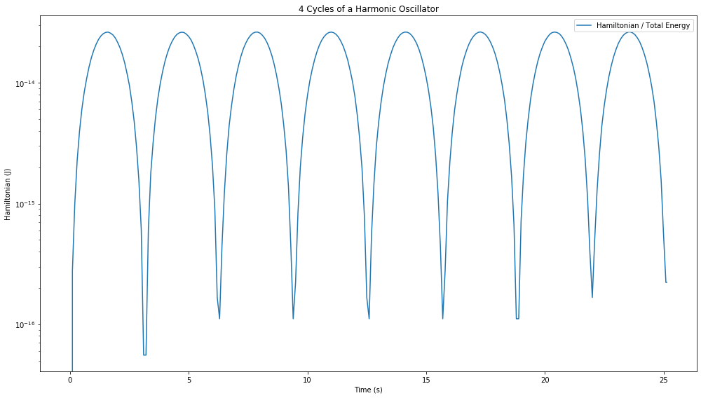
Well that’s completely different behaviour to the adaptive integrator. We see now that the Hamiltonian oscillates between a maximal error and a minimal one, but remains within \(10^{-14}\) of the true Hamiltonian. This is exactly the behaviour we were expecting. Let’s look further long term and compare with the adaptive integrator, we’ll decrease the adaptive integration tolerances down to \(10^{-12}\) to see if that helps.

fig = plt.figure(figsize=(14,8))
ax  = fig.add_subplot(111)

a.tf = 1024*2*D.pi

a.reset()
a.set_method("BABS9O7H")
a.dt   = 1e-1
a.integrate()

E_H = D.abs(hamiltonian(a.t, a.y.T, **a.constants) - hamiltonian(a.t[0], a.y[0], **a.constants))

disp_H = ax.plot(a.t, E_H, label="BABS9O7H", color='C0')

a.reset()
a.set_method("RK45")
a.rtol = 1e-12
a.atol = 1e-12
a.dt   = 1e-1
a.integrate()

E_H = D.abs(hamiltonian(a.t, a.y.T, **a.constants) - hamiltonian(a.t[0], a.y[0], **a.constants))

disp_H = ax.plot(a.t, E_H, label="Runge-Kutta 45", color='C1')

a.reset()
a.set_method("RK87")
a.rtol = 1e-12
a.atol = 1e-12
a.dt   = 1e-1
a.integrate()

E_H = D.abs(hamiltonian(a.t, a.y.T, **a.constants) - hamiltonian(a.t[0], a.y[0], **a.constants))

disp_H = ax.plot(a.t, E_H, label="Runge-Kutta 8(7)", color='C2')

a.reset()
a.set_method("RK108")
a.rtol = 1e-12
a.atol = 1e-12
a.dt   = 1e-1
a.integrate()

E_H = D.abs(hamiltonian(a.t, a.y.T, **a.constants) - hamiltonian(a.t[0], a.y[0], **a.constants))

disp_H = ax.plot(a.t, E_H, label="Runge-Kutta 10(8)", color='C3')

a.reset()
a.set_method("RK1412")
a.rtol = 1e-12
a.atol = 1e-12
a.dt   = 1e-1
a.integrate()

E_H = D.abs(hamiltonian(a.t, a.y.T, **a.constants) - hamiltonian(a.t[0], a.y[0], **a.constants))

disp_H = ax.plot(a.t, E_H, label="Runge-Kutta 14(12)", color='C4')

ax.set_xlabel("Time (s)")
ax.set_ylabel("Hamiltonian (J)")

# added these three lines
ax.legend(loc='lower right')
ax.set_yscale("log")

ax.set_title("{:.0f} Cycle{} of a Harmonic Oscillator".format(a.tf/(2*D.pi), "s" if a.tf/(2*D.pi) > 1 else ""))
plt.tight_layout()

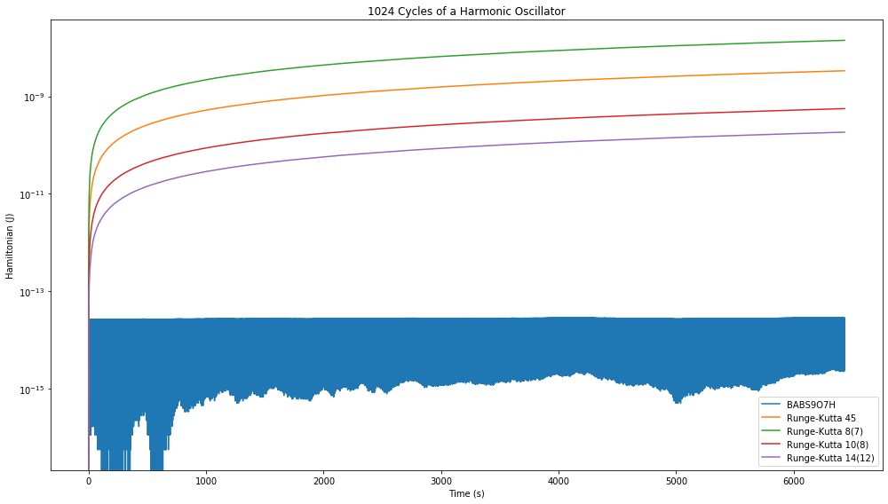
That’s not good, the Hamiltonian error increases consistently with continued integration whereas the 7th order symplectic integrator continues to stay bounded.

Thus we see that if energy conservation is a concern, then a symplectic integrator should be used. In most cases, the adaptive Runge-Kutta methods are more useful as they generally require fewer function evaluations and give very good results.